The key to science is reproducibility: if others can’t check your work, it might as well not exist.
This idea is evolving into a concept called reproducible research: don’t just publish the results of an analysis, publish the analysis itself—including the raw data and software. This accelerates progress: providing working code makes it easier to verify the results, and easier to build on them.
This applies to scientific blogging, too. Blogs are already a fast way to spread ideas. Blogs with data and software included—“reproducible blogs”—are even faster. Not to mention, it’s harder for mistakes to hide.
Tips for reproducible blogging with knitr
I’ve set up this website to support reproducible blogging. Here are some of the things I’ve learned along the way.
Use a static site generator
Dynamic sites build the page every time it loads. Static sites are nothing more than simple HTML files. For reproducible blogging, static sites have the edge.
Re-running the R code every time the page loads would be too slow (and probably technically infeasible). Instead, run the code locally on your computer, and just generate the HTML files once. This also makes hosting much easier: you don’t need special software like PHP and MySQL; literally any webserver will do.
My weapon of choice is nanoc. It’s very actively developed, and it’s flexible and extensible enough to handle whatever tools I want to use. The downside (for me) is that it’s written in Ruby, and I don’t know Ruby. But I’m glad I didn’t let that stop me; in practice, it’s been easy to pick up just what I need.
Automatically link to the source for every page
True transparency doesn’t make people hunt. It advertises!
In my case, I put a link at the top right of each page to its own source. Here’s how I did it in nanoc.
Think of knitr as a text filter
In other words: a thing which gets some input text, modifies it, and outputs the result.
The knitr filter has one simple job: run the snippets of R code it finds, and stick the results in the text. It doesn’t need to worry about other manipulations, since filters can be chained: the output of one is the input of the next. For instance, I use a pandoc filter to turn the output of knitr into HTML for my website.
Don’t be scared by git’s lousy image handling
I procrastinated for more than a year between writing that knitr filter and adding support for figures. The bogeyman was git’s awful reputation for handling image files. Over the years, people have developed a confusing array of not-quite-satisfactory workarounds. I didn’t want to go through the hassle of comparing them and committing to one.
Happily, git’s handling of images turns out to be a complete non-issue, since the images never end up in git.1 Only the source code goes in version control. The output (including images) just gets copied to the webserver.
I wish I’d realized sooner how easy it was! I could have been making beautiful plots for years.
Set base.path to the output directory for your post
If we want figures, the simple “filter” model isn’t enough. Instead, knitr becomes a “filter with side effects”. Here’s what I mean.
Sometimes, an R snippet does more than simply output an answer; for example, when you construct a plot, it creates an image file. That image is the “side effect”. And it raises a question: where should that file be created?
Clearly, it needs to be created somewhere under the output/ directory, or else it won’t end up on the webserver when we copy the files over. If we want to keep things neat (and if we don’t want to worry about filename collisions!), we should probably stick it in a subdirectory specific to its post.
Fortunately, knitr has an option called base.dir which controls where the figures end up. Getting the figures right is as simple as setting this option to the appropriate directory for the current post.
Don’t be confused by the similarly-named root.dir option! For purposes of getting the figures to work, it’s a complete red herring.
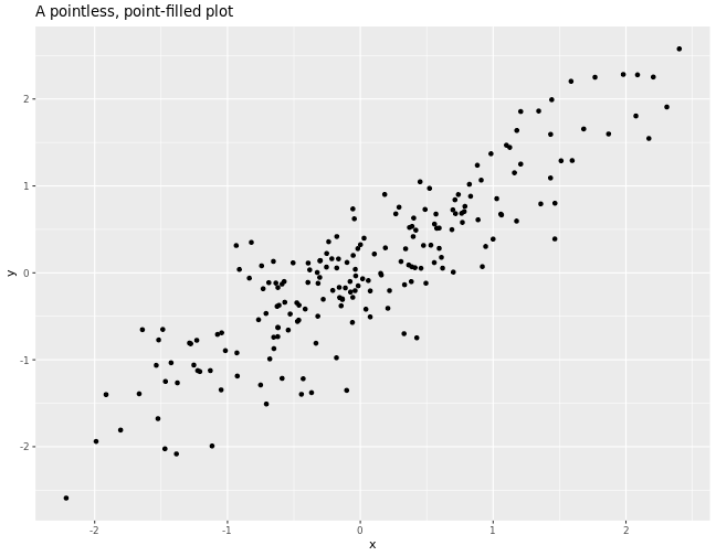
A simple example
# Fix the seed for the random number generator (for reproducibility).
set.seed(1)

# Let's generate 200 pairs of random numbers.
N <- 200
random_numbers <- matrix(ncol=2, rnorm(n=2 * N))

# Generate a simple covariance matrix, and take its Cholesky decomposition so
# we can use it to generate correlated random draws.
covariance <- matrix(c(1, 0.9, 0.9, 1), nrow=2)
cholesky <- chol(covariance)
d <- data.frame(random_numbers %*% cholesky)
names(d) <- c('x', 'y')

# Make a simple scatterplot.
require(ggplot2)
print(ggplot(data=d, aes(x=x, y=y))
      + geom_point()
      + ggtitle("A pointless, point-filled plot")
      )
Join the fun!
I am far from the first to advocate and implement reproducible research in blogging. For example, Carl Boettiger has maintained an open lab notebook for years, and I’m sure there are many other examples which I haven’t yet seen.
But I don’t want it to be merely possible; I want it to be commonplace. I want it to be standard. I want a world where it’s so easy to do it right, people are suspicious of bloggers who don’t. Sharing my implementation (and the tricks I learned along the way) is my modest contribution to making that world a reality.