The Cholesky decomposition is a key concept in matrix algebra. It’s a kind of “matrix square root”: a lower-triangular matrix \(L\) which gives back the original matrix \(K\) when multiplied with its transpose: \[L L^\intercal = K.\]
It’s very useful for working with high-dimensional Gaussian distributions. \(L\) takes independent one-dimensional Gaussian samples (i.e., the simplest possible case), and turns them into samples from the multidimensional distribution whose covariance matrix is \(K\).
For example, take the highly-correlated matrix \[K = \left[\begin{array}{cc}1 & 0.8 \\ 0.8 & 1\end{array}\right].\] Its Cholesky decomposition is \[L = \left[\begin{array}{cc}1 & 0 \\ 0.8 & 0.6\end{array}\right],\] as we can easily verify: \[L L^\intercal = \left[\begin{array}{cc}1 & 0 \\ 0.8 & 0.6\end{array}\right] \left[\begin{array}{cc}1 & 0.8 \\ 0 & 0.6\end{array}\right] = \left[\begin{array}{cc}1 & 0.8 \\ 0.8 & 1\end{array}\right] = K.\] If we now use \(L\) to multiply independent normal samples, it turns them into correlated samples with a correlation of 0.8.
num_points <- 200
independent_random <- matrix(nrow=2, rnorm(n=2 * num_points))
correlated_random <- L %*% independent_random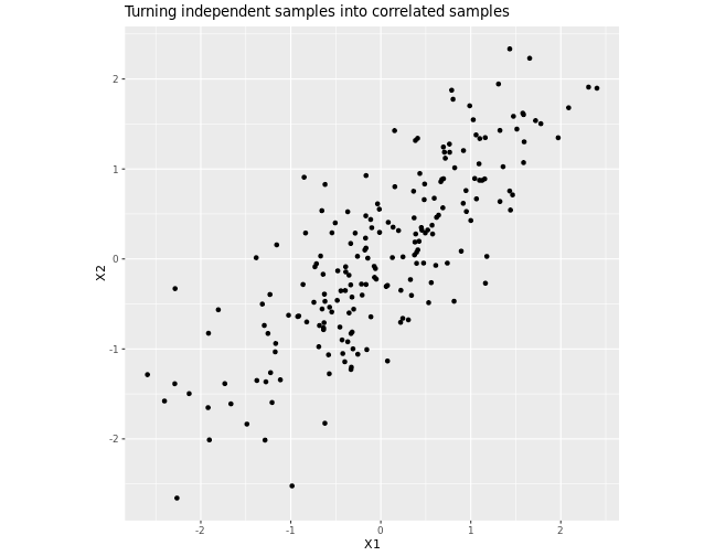
What’s missing in the above is any notion of how to calculate \(L\), given \(K\). If we have a good software library, we can just use it, and treat this calculation as a black box. But if we want to dig deeper, we’re in luck: it turns out we already have enough information to compute it from scratch.
Everything here is elementary, and I’m sure it’s quite well known. I’m only blogging it to share my utter delight when I stumbled across its underlying simplicity.
Adding “one more row”
In the appendix for my animation paper, I asked the question: given \(n\) draws from a Gaussian with a particular covariance function, can we efficiently compute the \((n+1)\)st?
If we have the first \(n\) draws, that means we have their covariance matrix \(K_n\) and its Cholesky decomposition \(L_n\), so that \(L_n L_n^\intercal = K_n\). We also have the covariance of every old point with the new point, a vector we’ll call \(k_n\), as well as the new point’s variance \(\sigma_{n + 1}^2\). Together, these form the new covariance matrix1, \[ K_{n + 1} = \left[\begin{array}{cc} K_n & k_n \\ k_n^\intercal & \sigma_{n + 1}^2 \end{array}\right] \]
What we need is the new row that makes \(L_n\) into \(L_{n + 1}\), where \(L_{n + 1} L_{n + 1}^\intercal = K_{n + 1}\). We can break this row into two pieces: a vector \(\ell_n^\intercal\) (corresponding to contributions from all the old points), and a scalar \(\gamma_{n + 1}\) (corresponding to the new point). This gives us a block matrix equation: \[ \left[\begin{array}{cc} L_n & 0 \\ \ell_n^\intercal & \gamma_{n + 1} \end{array}\right] \left[\begin{array}{cc} L_n^\intercal & \ell_n \\ 0 & \gamma_{n + 1} \end{array}\right] = \left[\begin{array}{cc} K_n & k_n \\ k_n^\intercal & \sigma_{n + 1}^2 \end{array}\right] \] What interesting equations fall out of this?
- \(L_n L_n^\intercal = K_n\)
- Well, we knew that already.
- \(L_n \ell_n = k_n\)
-
Now, this looks promising! \(L_n\) and \(k_n\) are known, so we can solve for \(\ell_n\).
It gets better: remember that \(L_n\) is lower-triangular, so the equation looks something like this: \[ \left[\begin{array}{cccc} L_{11} & 0 & 0 & \cdots \\ L_{21} & L_{22} & 0 & \cdots \\ L_{31} & L_{32} & L_{33} & \cdots \\ \vdots & \vdots & \vdots & \ddots \\ \end{array}\right] \left[\begin{array}{c} \ell_1 \\ \ell_2 \\ \ell_3 \\ \vdots \end{array}\right] = \left[\begin{array}{c} k_1 \\ k_2 \\ k_3 \\ \vdots \end{array}\right] \] (Everything is known except the \(\ell\)s.)
In the first row, \(\ell_1\) is the only unknown; we have \(\ell_1 = k_1 / L_{11}\). The second row uses only \(\ell_1\) and \(\ell_2\), but we already solved for \(\ell_1\): again, only one unknown, which is easy to solve.
Going down the line, we can solve for every element of \(\ell\), without even doing any matrix manipulations.
- \(\ell_n^\intercal \ell_n + \gamma_{n + 1}^2 = \sigma_{n + 1} ^ 2\)
- Since we already figured out \(\ell_n\) above, and we know \(\sigma_{n + 1}\), this equation is just as easy as the previous ones.
So: yes, we can compute the next row of the Cholesky decomposition if we know all the previous rows.
This smells like induction
We now know how to get \(L_{n + 1}\) if we have \(L_n\), but how do we get \(L_n\) in the first place? One way is to call a library function—always a good default strategy. This works pretty well, until it doesn’t.
Another approach would be to start with \(L_{n - 1}\), and use what we just figured out to add the final row. Of course, then we’d need \(L_{n - 1}\), but we could get it from \(L_{n - 2}\)…
At this point, I’m reminded of mathematical induction: a method to generate “valid for any positive integer” proofs based on two ingredients. One ingredient is a method for getting from step \(n\) to step \((n + 1)\) for any \(n\); we have that already. The other ingredient is a base case: an answer for the smallest possible \(n\) which doesn’t depend on any earlier stages.
In our case, the base case turns out to be trivial. The simplest matrix which could have a Cholesky decomposition is a \((1 \times 1)\) matrix; let’s say \(K = \left[ k \right]\) for some \(k > 0\). Then \(L = \left[ \sqrt{k} \right]\)—what could be easier!
We can put this all together to compute the elements of \(L\) one at a time. Each new element uses \(K\) and the elements of \(L\) we’ve already computed. Let’s update our notation for consistency: we’ll replace the \(\ell\)s and \(k\)s with the corresponding indices in \(L\) and \(K\). The matrix equation for a typical intermediate stage looks like this: \[ \left[\begin{array}{cc} L_{11} & 0 \\ L_{21} & L_{22} \end{array}\right] \left[\begin{array}{c} L_{31} \\ L_{32} \end{array}\right] = \left[ \begin{array}{c} K_{31} \\ K_{32} \end{array} \right] .\] This gives us the “pre-diagonal” elements of the third row, \(L_{31}\) and \(L_{32}\). We’ll then get \(L_{33}\) in terms of \(K_{33}\) and these same pre-diagonal elements, and this gives us everything we’ll need to compute the fourth row. So it goes, until we have the whole matrix.
I started out trying to extend existing Cholesky matrices, and I got the ability to compute any Cholesky matrix thrown in for free.
Testing it out
Let’s turn these ideas into actual code.
# This doesn't check that K actually *has* a Cholesky decomposition (not every
# matrix does).  Give it some garbage, and it will happily return a nonsense
# answer (if it doesn't crash first!).
#
# That's OK; the point is to see if it gives the right answer for suitable
# matrices.
#
# For this reason (and many others!), you shouldn't be using this algorithm in
# the real world: like the blog post it's part of, it's only good for improving
# your understanding of the concept.
MyCholesky <- function(K) {
  n <- nrow(K)

  # Start out with a matrix which is all zeroes, except for the upper-left
  # element.  (We know that element is the square root of the corresponding
  # element in K, since that's the base case.)
  L <- matrix(0, nrow=n, ncol=n)
  L[1, 1] <- sqrt(K[1, 1])
  if (n == 1) { return(L) }

  # Compute each row's values.
  for (row in 2:n) {
    # This loop computes all the elements *before* the diagonal (which
    # corresponds to step 2 above).
    for (col in 1:(row - 1)) {
      # sum_to_subtract is the contribution of the elements we've previously
      # computed in this new row.
      sum_to_subtract <- 0
      if (col > 1) {
        i <- 1:(col - 1)
        sum_to_subtract <- L[col, i] %*% L[row, i]
      }
      L[row, col] <- (K[row, col] - sum_to_subtract) / L[col, col]
    }
    # Now compute the element on the main diagonal (corresponding to step 3
    # above).
    i <- 1:(row - 1)
    L[row, row] <- sqrt(K[row, row] - L[row, i] %*% L[row, i])
  }
  return (L)
}
To test this, I’ll construct a random \((20 \times 20)\) covariance matrix. I’ll compute its Cholesky decomposition twice—once with my method, and once with R’s built-in chol() function—and see how close the two answers are.
# Generate some points.
x <- sort(rnorm(n=N))

# Construct a matrix from a covariance function which I know is valid.
# (We'll add some noise on the diagonal to help it converge).
K <- outer(x, x,
           function(a, b) {
             exp(-(a - b)^2) + ifelse(a==b, 0.01, 0.0)
           })

# What are the biggest and smallest differences between my method,
# and R's built-in method I know is correct?
range(MyCholesky(K) - t(chol(K)))
## [1] -1.915135e-15 2.720046e-15So the biggest difference was smaller than \(10^{-14}\). Looks pretty good to me!
Conclusions
Don’t be intimidated by theorems with hard to pronounce names. They often contain extremely simple ideas.